 Mgt 3325 -
Home Spring 2010
Email
to Dr. Lyons
PatLyons Home
Mgt 3325 -
Home Spring 2010
Email
to Dr. Lyons
PatLyons Home
[ Calendar12:20 |
1:25
| Class Participation AI | App of OM |
Table of Contents | Search ]
[ Ch 1 | 2 |
3 | 4 | 5
| 6 | 6S |
7 | 8 | 9 | 10 | 11
| 12 | 13 | 14
| 15 |
16 | 17 | | HW1 | 2 | 3
| 4 | | Career1| 2
| 3 | 4
]
[
SJU
|
TCB |
CareerCenter |
StudentInfo |
CareerLinks |
Internships ] [NYC Teaching
Fellows] [
SJU Closing ] [H1N1SelfAssessment]
Ch 12 - Inventory Management
- Introduction
- Def - Inventory - any resource held for future use
- Functions of inventory
(p484)
- *Decoupling - when two processes cannot be synchronized, inventory can smooth
fluctuations. Example, firm with high seasonal demand, produces some products in
off-season.
- Quantity discounts
- Hedge against inflation
- Types of Demand (p489)
- Independent demand - typical finished product - demand from many small
independent customers
- Dependent demand - typical component of a finished product - demand for lawn
mower wheels is dependent on demand for lawn mowers. (Ch 14 - Material Requirements
Planning)
Basic Economic Order Quantity (EOQ) Model (p490)
- Def - EOQ - the order quantity which minimizes total ordering and holding costs.
- Assumptions
- Uniform demand
- Replenishment of Q units arrives as last unit is used
These assumptions imply (see Fig 12.3)
Avg inventory level = Q/2
- Costs
- Annual ordering (set-up) cost - preparing order, (setting up process), receiving
shipment, placing in inventory.
= S (D / Q)
S - ordering (set-up) cost for each order
D - annual demand
Q - order quantity
- Annual holding cost - storage, taxes, investment, insurance, obsolescence (see
Table 12.1, p490)
= H (Q / 2)
H - holding (carrying) cost per unit per year
Q/2 - average inventory level
- Fact: EOQ occurs when ordering cost = holding cost.
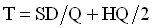
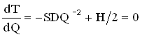
Implies
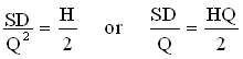
- *EOQ
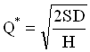
- See Example 3 - page 493
Do
assigned HW
Probabilistic Models
Definitions
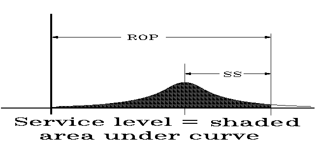
- Safety stock - extra stock carried to reduce the probability of stockout due to:
· unexpectedly high demand during lead time and/or
· unexpectedly long lead time
- DL - random variable denoting demand during lead time
- ROP - reorder point - inventory level (point), at which order is placed
ROP = mean(DL) + safety stock
- *Service level - probability of supplying stock during lead time
service level = Prob( DL Ł ROP )
Memphis Regional Hospital - page 504
- Determine the safety stock, if the desired service level is 95%.
- DL is normally distributed with a mean, µ, of 350 and a standard
deviation, s, of 10.
- Let SS denote safety stock and Z = ( DL - µ ) / s.
- Then, service level = Prob( DL Ł ROP ) =
Prob( Z Ł SS/s )
- From Appendix I, page A2, Z1 = 1.65 satisfies Prob(Z Ł Z1) = 0.95
- Therefore, safety stock = Z1 s = 1.65 (10) = 16.5
ROP =
mean(DL) + safety stock = 350 +
16.5 rounded up to 367 units
Do assigned HW
Independent Demand Inventory Systems
*Fixed-quantity System
- Procedure
Establish order quantity, Q, and reorder point, ROP
Review inventory level, I, with each transaction
If I Ł
ROP
then order Q.
- Advantage (compared to fixed-period system)
Lower probability of stockout
- Disadvantages
Requires perpetual record keeping
Numerous independent orders
*Fixed-period System (p507)
- Procedure (Fig 12.9)
Establish max inventory level S
Review inventory level, I, at intervals of T (every
week or month or . . . )
Order S-I units on each occasion.
- Advantage (compared to fixed-quantity system)
Consolidation of individual orders
- Disadvantage
Possible small individual order size
*ABC Analysis
(p485)
- Procedure
- List inventory items by decreasing value (annual dollar usage, investment,
profit, . . .)
- Group items into classes (slightly different than textbook)
- Class A contains items in top 70% of
value
Typically Class A contains 10-20% of inventory items
- Class B contains items in middle 20%
of value
Typically Class B contains 20-35% of inventory items
- Class C contains items in bottom 10%
of value.
- See Example 1 - Silicon Chips
- Worksheet for Client ABC Analysis -
click here to download my worksheet,
ABCAnalysis.xls.
- Typical use
| Establish: |
Possible Inventory System: |
| Tight control on A items |
Fixed-quantity |
| Moderate control on B items |
Fixed-period (computerized) |
| Loose control on C items |
Fixed-period (manual) |
(This page was
last edited on
October 22, 2009
.)